Energy Environment and Economy

1. Introduction

In Iraq, water shortages and energy shortages have come together. These two problems are arising combinedly and makes morse each other and this problem cannot be overlooked.  Due to the building of dam in upstream on the Tigris and Euphrates causes the reduction of surface water lower stream, which is the real scenario of water resources management in Iraq (Al-Khatib & Al-Sari, 2021).

The arable land becomes salinization because of low and decreasing rainfall and dry season in the different provinces of Iraq (Mahmoud, 2022). These two problems are corelated and lack of surface water introduce the more demand of groundwater, which also required energy to pump and getting the groundwater for agricultural purposes. These overall scenario effect the livelihood pattern of rural people. When the power supply is not sufficient it may concern for the groundwater collection.

Babylon Governorate also experienced the unusual conditions, in the Al-Shamali the surface water and energy supply for groundwater pumping is a major concern. Most groundwater extraction depends on the diesel generator (Al-Saffar, 2020). As a result of surface irrigation is not consistence which impact on grid electricity and as well as the energy supply for groundwater extraction.

The overall process for diesel generator is well accepted but the problem is the process of oil and fluctuating besides this the generator needs to regularly repair and bear the maintenance cost as it has bee be work in the open places under dry and hot with dusty weather. Another big impact of the generator is producing green house gasses which is ultimately causes impacts on the environment. So, the alternative sustainable and environmentally friendly option need to search for which will be also economically viable.

Solar photovoltaic (PV) technology is a outstanding alternatives to meet the all criteria of benefits, scientist have discovered that how sunlight can be turned into useful electrical energy to run the pump to extract groundwater from few decades ago (Duffie & Beckman, 2013; Goetzberger & Hoffmann, 2005).

The researchers are trying to find out the precise system or design for specific water pumping load to run for water supply as a alternative for diesel generator. Glasnovic and Margeta(2007) claimed that solar pumping will be the best option when sunlight pattern is matched to the irrigation demand.  There are many studies agreed with them that the solar pumping process is exceptional and more reliable pathways. , Chandel and Nagaraju (2015) research find out that small local PV pumping systems loss less energy in compare with a large setting. Kumar and Rosen (2017) conduct a broad review and demonstrated that large systems are more energy consuming as a result the system designer think small size may be effect on the systems performances. The large size of energy systems may cost extra charge on maintenance and not reliable. This is the main reason not to used the technology more quickly for water pumping.

In the solar panel and solar pumping system one of the more important issues is hoe many power is taken from the solar panel to chose the the right size of the system is describe by Hamidat et al. (2003), they also mention that when sunlight is weak or the panel is partly dark the load must be adjust constantly, without this the pump may not be working properly and do not give the best output.  In the PV pumping system maximum power point tracking (MPPT) is standard for well design PV pumping system. Software such as PVsyst and MATLAB make it easier and more convenient to predict the interaction of the Panel and pumps Khatib & Elmenreich, 2016; Ibrahim & El-Mahdy, 2018). Software simulations is helpful but cannot fully detect what is happening in the real environment especially when the dust effect, sunlight heat is disturbing etc. Overall, the renewable energy research in Iraq is enhancing but it is still not fulfilling the demand.  To improve the performance of the solar powered pumping systems MPPT is working like a superhuman in the well-designed system. Besides this PVsyst and METLAB like thse software also help to predict about how the solar panel and Pump work together before installing and starting performance (Khatib & Elmenreich, 2016; Ibrahim & El-Mahdy, 2018). 

Al-Saffar (2020) and Al-Khatib and Al-Sari (2021) has done researches on different types and categorizations of considerable solar resources potential and renewable energy capacity available to decrease the load of energy from the nation grid. The findings from the Mahmoud (2022) clearly mention about that specifically advantages of solar power irrigation over the diesel pump. There is very few studies on these comparisons. Theoretical and simulation in pump installation is important but practical field installation with measured performance data based on generalized climate related strategies help more better for the performance of the pump setting to get the best performance in different condition of the different region of the country.

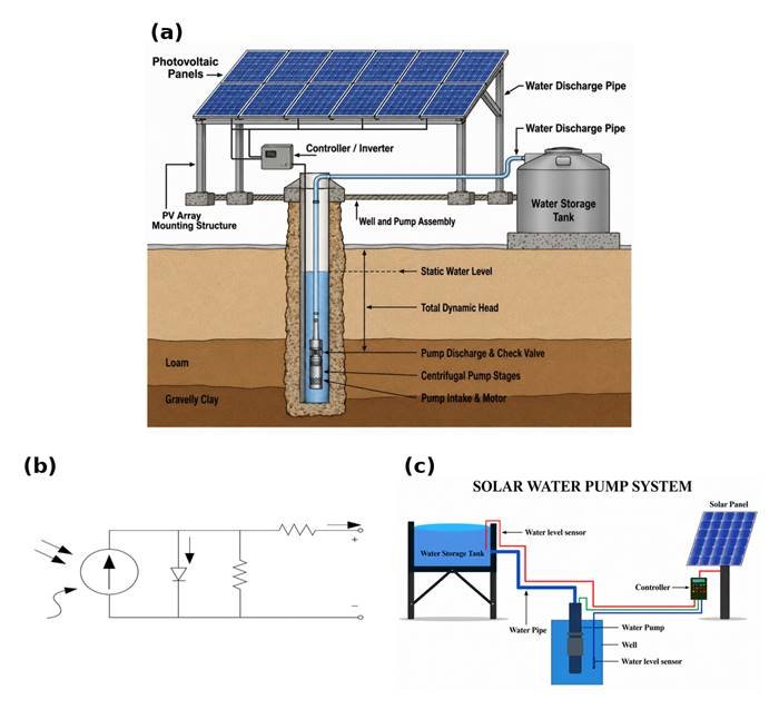
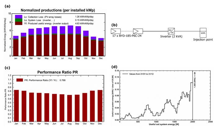
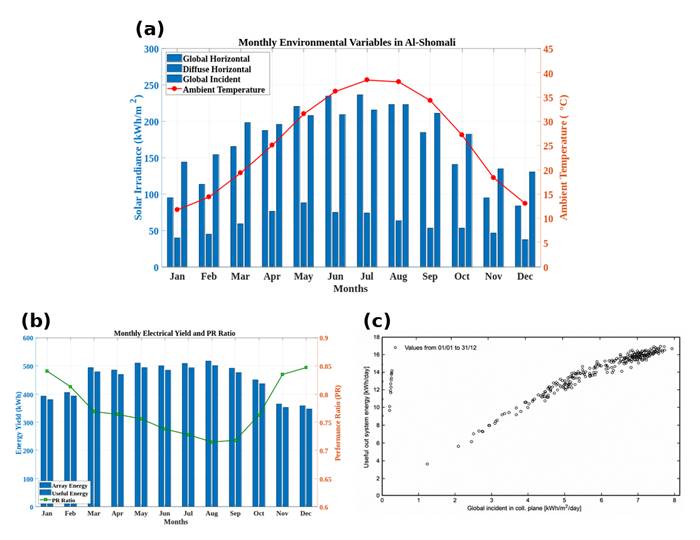
This study tries to find out these research gap. In this study hydraulic and electrical design of a standalone 1500 W PVWPS are designed to the specific conditions of Al-Shomali districts of Iraq. The design was followed a PVsyst simulation built on local meteorological inputs and which is most useful to predict the measurement This study will give a clear reasonably transparent reproducible account of how this type of system perform and meets the environmental conditions of the environment of Summar in Iraq.

2. Methodology

2.1 Study Design and Site Description

In this research we have used three main steps which are: system design, computer simulations, and field testing. For the measuring the requirement of the system, first we have done the hydraulic and electrical calculation. Next computer software was used to predict how the system would perform. Finally, the system was installed at an agricultural site and its performance was measured under actual operating conditions.  The study was conducted on a working agricultural farm in the AL-Shomali district of Babylon Governorate, Southern Iraq. The exact geographical coordinates and elevation of the study site also provided. The region has an arid to semi-arid climate with very hot summers and high levels of solar radiation. Farmers mainly depend on groundwater from artesian wells for irrigation because surface irrigation cannels in the area no longer provide a reliable water supply.   

2.2. Water Demand and Hydraulic load determination

The daily water demand for agriculture ((V)) was set at 25 m³/day. This amount was estimated based on crop water needs, soil evaporation and the cultivated area supplied by the wall. The author should specify the crops types cultivated areas in hectors and the methods used to calculate references evapotranspiration, such as the FAO penman- Monteith method, so that other researchers can verify the estimate. The total Dynamic Head (TDH) represents the total height and resistance that the pump was selected to draw water from an artesian well with an operating depth of approximately 25-30 m and a borehole diameter of 15 cm.

The Total Dynamic Head (TDH) represent the total height and resistance that the pump must overcome to deliver water to the storage tank. It was calculated by adding four components. According to the standard hydraulic relation.

TDH = H_static + H_drawdown + H_discharge + H_friction (1)

Here H is the static water in the well, measured at 18 m. The author should specify the instrument used for this measurement. H_drawdown is the additional drop in he water level during pumping, estimated at 4 m. The merhod and duration of the well test used to determine this value should be reported. H discharge is the vertical distance from ground level to the tank inlet, measured at 3 m. H friction represent the head loss caused by friction in the pipes and fittings, calculated methods, such as the Hazen-williams or Darcy-Weisbach equation.  Using these values the total dynamic head was calculated as TDH = 18 + 4 + 3 + 2.5 = 27.5 m, which was then used as the design basis pump selection and PV array sizing.

2.3 Electrical and Hydraulic Energy Sizing

The required daily hydraulic energy (E_h. kWh/day) needed to lift the design volume against the calculated TDH was obtained from the standard fluid-mechanics relation

E_h = (ρ · g · V · TDH) / (3.6 × 10⁶) (2)

Which for water (ρ= 1000 kg/m³) and standard gravitational acceleration (g=9.81m /s²), simplifies to the commonly used engineering approximation

E_h = (V · TDH) / 367 (3)

In the design parameters equation 3 was applied (V = 25 m³/day, TDH = 27.5 m) yields a net hydraulic energy demand of approximately 1.87 kWh/day. Because this figure represents only the theoretical minimum, it does not account for real word lossess in the pump motor, and any power conditioning electronics. The required photovoltaic array energy (E_PV) was therefore derived by dividing the hydraulic energy by an assumed overall system efficiency.

(η_sys):

E_PV = E_h / η_sys (4)

A conversion of η_sys of 45-50% was adopted, reflecting typical electromechanical lossess under high-temperature field conditions. Which supported the selection of a 1500 W array- a margin intended to accommodate soiling losses, thermal derating in summer and day to day irradiance variability rather than to meet the bare theoretical minimum alone.

2.4 System components and Configuration

There are five 300 W monocrystalline silicon panel were combinedly installed in a series pattern in the Solar array.  Under Standard Testing Conditions (STC) every panel has provided a voltage of 32.2 V and a current of 9.3 A. The all five panels provided a total power of 1500 W with an output voltage intended to fall within the operating range of the MPPT controller

The panels were installed on a fix metal frame with a tilt angle of 33° and an azimuth angle of 0°  (true south). These angles were selected to provide suitable solar exposure based on the location latitude

 A perturb and observe (P&O) maximum power point tracking (MPPT) methods was used to help the system obtain the maximum available power from the solar panels as sunlight changed. The author should specify the controller’s manufacturer, model firmware and operating parameters, including the voltage adjustment steps and sampling interval. The system was designed to operate according to the available solar power. This approach was intended to reduce the risk of pump stoppage during periods of low sunlights or partial shading  Water level sensors were installed in both the wall and the storage tank. These sensors provided information to the control system to help prevent the pump from running without suffucuent water and to stop pumping when the 25 m³ storage tank was full.

The system did not used batteries to store electrical energy, instead water stored in the tank served as a reverse for periods without sunlight.  This arrangement reduced the need for batteries storage although the available water supply depends on the tank’s capacity and the amount of water pumped during daylight hours. The limitations of this design are discussed in a later section.

2.5 Simulation Protocol

Performance simulation was conducted using PVsyst (PVsyst SA, 2024). Hourly weather dta for the AL Shomali study site were used as input. The author should specify the source of these data such as the Meteonorm database satellite based solar radiation data or measurement from a local weather station. We checked the data collection period and time resolution. We developed the solar array model without any shading or horizon problems. The software device library provided the electrical characteristics of the  solar panels MPPT controller settings and pump performance curve. This was associated with datasheets from manufacturers.

The seasonal changes in solar radiation and ambient temperature and their effect on the water pump determined for one year with our simulation model. The system loss data and performance ration determined with the obtained data shown in the results section.

 2.6 Field Deployment and Empirical Validation Protocol

We installed the practical simulation model to determine its activity at the study location as per our system conditions. We determined the water flow rate with a calibrated 1 m3 tank and a digital timer.

Measurements were taken at the design operating point, with a total dynamics head (TDH) of 27.5 m. To ensure that the results could be reproduced the author should report the number of measurement trial, test dates and times of day.

We observed the activity of the simulated model with a real system to demonstrate the performance.  The specified monitoring period, including the start and the end dates. The Performance Ration (PR) for daily water flow was added in the analysis. The system performance and its efficiency was tested under different seasonal conditions.

When differences between simulated and measured performance were observed dust accumulation on the solar panels was considered a possible contributing factor. Dust can reduce the amount of sunlight reaching the panels and lower their power output. However, the effect of dust was assessed qualitatively in this study. Further research could measure this effect more accurately by comparing the output of clean and dusty panels under similar environmental conditions

2.7 Environmental and Performance Metrics

The performance of the solar powered water pumping system was evaluated using four indicators: Performance Ratio (PR), overall system efficiency (η_sys), epecific energy yield (Y_f, kWh/kWp/day) and total annual pumped volume.

The performance ration was used to assess the system actual performance compared with its expected energy output. Overall system efficiency measured how effectively the system converted solar energy into useful pumping energy. Specific energy yield represented the daily energy output per kilowatt of installed solar capacity, while the annual pumped volume indicated the total amount of water supplied during the year.

The annual reduction in carbon dioxide (Co2) emission was estimated by comparing the solar -powered system with an equivalent diesel-powered pumping system. A diesel -generator emission factor of 0.8 kg Co2/kWh was used for thgis calculation based on the references cited in the original study (IPCC< 2006).

3. Results and Discussion

3.1 Annual Energy Yield and Overall System Efficiency

In the solar panel array in a one year, it received over all 2100 kWh/m2 of global solar radiation. The simulation of the panel by Software also calculated for one metrological year to find the reliable and best calculation output for the panel arrays. In the Table 1, The total useable energy was mentioned which is about 2800 kWh/year. This was the best output and has the benefits from the hydraulic sizing which is almost about to 25 m³/day. The simulation also helpto find out the real variability. The overall system efficiency was 48% mention in the Table 1. This value is typically for an electromechanical fluid transparent system. These also indicates the thermal losses in the array and further also mention the mechanical losses. 

 3.2 Seasonal Productivity and loss Distribution

The system is overall a predictable season covering a whole meteorological year. In the Figure 2a the normalized productivity analysis also present. The useful energy production (y_f) average 4.63 kWh/kWp/day. In the month of November to February the production has dropped due the heat of the sunlight availability because the winter has short daylight in compare to the summer season. The solar angle was low in these periods. The collection losses (L_c) averaged 1.26kWh/kWp/day. These losses were concentrated in the summer seasons because high module temperature occurred in that season. Monocrystalline cells have a negative temperature coefficient therefore part of the gain from the higher irradiance were lost. Ther energy availability and the thermal loss show an inverse seasonal relationship. This patterns common in hot climate reason.

The unused energy (L_u) in power generator is estimated at 1020kWh/day. In the Figure 2b the losses of energy are mentioned in details. The losses or unused energy substantially depends on the sizing of the systems. The oversizing was roughly around 120 W its purposes was to maintain output during the cloudy periods of times in the sky and the collection loss of the solar power pumps was estimated is around 0.85 kWh/day. They value are all acceptable for standardization, besides this the active energy of the pump was 2.95 kWh/day after the loss’s energy calculation.

3.3 Performance Ratio Stability

In the figure 2c the monthly performance Ration was mentioned, The PR stayed within a acceptable range which is calculated as 77% are 0.768. Due to the temperature and irradiance of local area a few changes are shown in the monthly calculation. The P&O, MPPT controller is contribute much and its significance is higher in compare with other topics. The controller continuously moved the pumps operating voltage because the combination of the array instantaneous maximum power point. This action shows the minimum performance losses. Partial shading and high summer temperatures therefore had a smaller effect.

3.4 Field Deployment and Array Configuration

The physical prototype is shown in Figure 1c, which is consisted of five series connected 300 W monocrystalline modules. Each module was estimated the at 32.2 V and 9.3 A at STC conditions. The angle for the module was kept at 33° angle and the same angle was used in the simulation by the software. The target flow rate of the solar powered pump was around 5000L/hour. This value was obtained from the daily demand of 25 m3 it also assumed five hours of useable insolation per day. We kept it simple with the plumbing layout. There were very few bends between the pump and the tank. We improved the design to avoid the extra friction loss in the system. Water level sensors were installed at the well and at the tank. The feedback from these sensors were essential. They protected the pump against dry running. When the tank was full, they turned off the pump as well. Figure 1c shows the overall ectro hydraulic architecture. The system was developed with the array controller and a storage tank.  An equivalent circuit of the single diode is shown in figure 1b. A bt PVsyst toll was added in the circuit to develop the model for the electrical behavior of the array.

3.5 Climatic Variability and Monthly Performance

Monthly climate data supports a point like solar irradiance and agricultural water demand peak at nearly the same time of year (Figure 3a). Ambient temperature peaks in the same window. Higher temperatures raise crop water demand, but they also lower PV efficiency.

Monthly electrical yield and performance ratio (PR), and their trends reflect this tension (Figure 3b). Energy generation is highest in midsummer, precisely when demand is greatest. PR dips over the same months, consistent with the thermal derating of monocrystalline silicon above the standard test condition (STC) reference

Figure 1. System architecture and field deployment of the standalone photovoltaic water pumping system (PVWPS). (a) Schematic block diagram of the electro-hydraulic components, showing the PV array, controller/inverter, well and pump assembly, and storage tank, with the Total Dynamic Head indicated. (b) Single-diode equivalent electrical circuit model of the deployed monocrystalline PV cell used for PVsyst modeling. (c) Electro-hydraulic integration diagram of the physical prototype as installed, showing water-level sensor placement, pump position, and pipe routing between the well, pump, and storage tank.

Figure 2. Simulated annual performance of the PVWPS over a full meteorological year. (a) Normalized specific productivity showing produced useful energy (Yf), collection losses (Lc), and system losses (Ls). (b) Simplified system component diagram used in the PVsyst loss model (array, inverter, injection point). (c) Monthly variation in Performance Ratio (PR), with an annual mean of 0.768. (d) Frequency distribution of the system’s useful output power across the annual operating cycle.

temperature. Even so, PR stayed fairly stable through this seasonal penalty, and that stability is arguably the more interesting result. It again points to the MPPT controller as the main stabilizing factor. derating of monocrystalline silicon above the STC reference temperature. Even so the remained fairly stable during this seasonal penalty. This stability is arguable the more interesting finding. It again points to the MPPT controller as the main stabilizing factor.

Figure 3c represent the useful energy and the incident radiation in a diagram, the relationship is linear as the operation points clustered closely along a single line. The pattern indicates that the MPPT algorithm always tracks the true maximum power point. The tracking did not show any major fluctuation or failure. It persisted for all ranges of observed irradiance conditions. 

3.6 Output Power Distribution and Equivalent Circuit Behavior

The annual distribution of the output power is shown in the Figure 2d. The system spends most of its operating time near the 1500W rating. The distribution is sharply packed at the high end of the power range. It was a unavailable environment but the array produced high efficiency output for most of the daylight hours

The distribution also has low frequency bands at the low power end. These bands represent short transition periods around sunrise and sunset. They also represent periods of heavy cloud cover. They don’t indicate any sustained underperformance. Figure 1b shows the single -diode equivalent circuit model. The model contains a light generated current source. It also contains a stunt resistance and a series resistance. These resistances represent ohmic and leakage losses. This model formed the basis of the PVsyst simulation of these dynamics. The series and shunt resistance values were especially important. They strongly shaped the response of the simulation I-V curve to the temperature and irradiance profile of Al-Shomali.

3.7 Field Validation Against Simulation

Volumetric field tests were carried out with a 1 m³ metering tank and digital timing at the design operating point of 27.5 m total dynamic head (TDH). The measured performance ratio (PR) was close to the simulated value of about 78% (Table 2). Because the measurement period was short, this result should be treated as an initial validation, not a long-term average.

The remaining difference between measured and simulated PR is most likely due to soiling. Fine dust settles on the panels almost daily in this part of Iraq, and some partial shading of the array by dust may also have contributed. The perturb-and-observe (P&O) MPPT controller helped throughout the day by adjusting the pump’s operating voltage to follow the maximum power point as irradiance changed, which prevented the pump from stalling.

3.8 Techno-Economic Implications

Taken as a whole, these results point toward a system that is not just technically functional but plausibly the more sensible economic choice over time, given the ongoing fuel, maintenance, and downtime costs associated with diesel alternatives (cf. Kumar & Rosen, 2017). That said, the present study did not carry out a formal levelized-cost-of-water or payback-period calculation, and doing so — ideally incorporating local diesel fuel prices, capital cost of the PV/MPPT/pump package, and expected maintenance intervals — would considerably strengthen the techno-economic claims made here and is recommended as a priority for follow-up work.

4. Conclusion

 This study designed a 1500 W standalone photovoltaic water pumping system for groundwater extraction using solar powered energy pump. It also simulated and field tested the system by software. The system served the AL-Shomali district of Babylon Governorate. It was sized to overcome a Total Dynamic Head of 27.5 m. It was also sized to deliver about 25m3 of water per day. The simulation results and field measurement are well fit for this system and pmp. The average performance ratio was close to 78%. The overall system efficiency was about 48%. The Perturb and observe MPPT controller appeared central to this stability. It helped the system cope with variable irradiance. It also helped with seasonal temperature swings. The system was estimated to avoid about 1.8 tons of Co2 per year compare with diesel pumping. These findings support one main conclusion: a carefully sized, site-specific photovoltaic water pumping system (PVWPS) can replace diesel-based irrigation reliably and at a reasonable cost. This conclusion applies to other region with scarce water and limited grid access. Further work is needed, particularly long-term monitoring across several seasons to confirm that the system

Figure 3. Field climatic conditions and empirical performance validation. (a) Monthly solar irradiance components (global horizontal, diffuse horizontal, global incident) and ambient temperature recorded at the Al-Shomali site. (b) Monthly electrical energy yield (array and useful energy) alongside monthly Performance Ratio. (c) Scatter relationship between daily global incident solar radiation and daily useful system energy output, illustrating the linearity of the array’s electrical response across the full range of irradiance conditions.

Table 1: Technical and physical specifications of the proposed PV pumping system in the Al-Shomali area.

Table 2: Analytical summary of annual simulation results and overall system performance indicators.

performs consistently throughout the year. A formal economic analysis would also help including payback period and LCOW    Such work confirms the durability of this solution at scale it would also confirm its cost effectiveness.

Acknowledgments

The author is grateful to the academic faculty who provided guidance throughout this research, and to the cooperative farmers of the Al-Shomali district for their practical support during field implementation.

Author Contributions

S.A.M.A.-H.: conceptualization, methodology, software, formal analysis, investigation, data curation, writing – original draft, writing – review and editing, visualization, project administration.

Funding

Self-funded research. No financial support or commercial grants were received during the preparation or execution of this study.

Competing Financial Interests

The author S.A.M.A.-H declares no competing financial interests, personal relationships, or commercial affiliations that could have influenced the work reported in this manuscript.

References